LinkedIn heavily relies on artificial intelligence to deliver content and create economic opportunities for its 575+ million members. Following recent rapid advances of deep learning technologies, our AI engineers have started adopting deep neural networks in LinkedIn’s relevance-driven products, including feeds and smart-replies. Many of these use cases are built on TensorFlow, a popular deep learning framework written by Google.
In the beginning, our internal TensorFlow users ran the framework on small and unmanaged “bare metal” clusters. But we quickly realized the need to connect TensorFlow to the massive compute and storage power of our Hadoop-based big data platform. With hundreds of petabytes of data stored on our Hadoop clusters that could be leveraged for deep learning, we needed a scalable way to process all of this information. Fortunately, TensorFlow supports distributed training, a useful technique for processing large datasets. However, orchestrating distributed TensorFlow is not a trivial task and not something that all data scientists and relevance engineers have the expertise, or desire, to do—particularly since it must be done manually. We wanted a flexible and sustainable way to bridge the gap between the analytic powers of distributed TensorFlow and the scaling powers of Hadoop.
Open sourcing TonY
To meet our needs, and because we know there are many others interested in running distributed machine learning who are also running large Hadoop deployments, we have built TensorFlow on YARN (TonY), which we are open sourcing today. Please check out the TonY project on GitHub for details on how to use it. Contributions and suggestions from the community are welcome!
In the rest of this blog post, we will cover the internal details of TonY, the features we have implemented and leveraged to scale distributed TensorFlow on Hadoop, and experimental results.
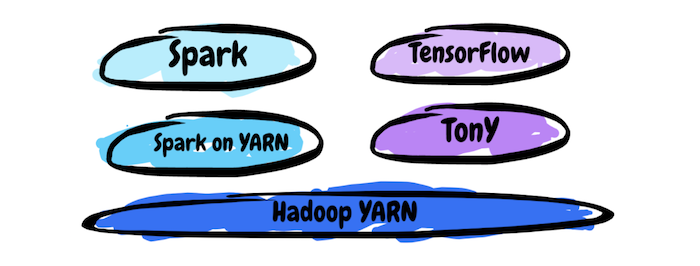
Existing solutions In our initial investigation into running distributed TensorFlow on Hadoop, we found a few existing solutions. However, we ultimately determined that none met our particular requirements, leading to our decision to build TonY.
TensorFlow on Spark is an open source solution that enables you to run TensorFlow on the Apache Spark computing engine. We were able to onboard a couple of our internal deep learning applications on this framework, but ran into a few issues, most notably a lack of both GPU scheduling and heterogeneous container scheduling. Also, any scheduling and application lifecycle enhancements we wanted to make in the future would have to be done in Spark, which is much more difficult than making the change in a self-contained YARN application.
TensorFlowOnYARN is another open source solution that runs as a separate library. Unfortunately, fault tolerance support and usability in this project did not fit our needs. Furthermore, this project is no longer maintained.
For these reasons, we decided to build TonY to give us complete control over the resources in our Hadoop clusters. Also, since TonY is running directly on YARN and runs as a lightweight dependency, we can easily evolve it with both the lower-level part of the stack in YARN, or the higher-level part of the stack in TensorFlow.
How does TonY work?
Similar to how MapReduce provides the engine for running Pig/Hive scripts on Hadoop, and Spark provides the engine for running scala code that uses Spark APIs, TonY aims to provide the same first-class support for running TensorFlow jobs on Hadoop by handling tasks such as resource negotiation and container environment setup.
Running TensorFlow on TonY on YARN
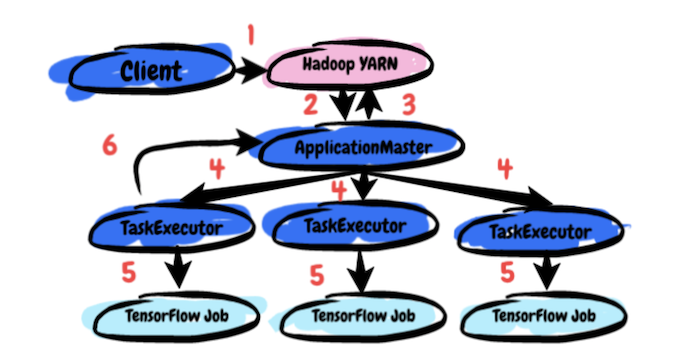
There are three main components to TonY: Client, ApplicationMaster, and TaskExecutor. This is the end-to-end process of running a TonY job:
The user submits TensorFlow model training code, submission arguments, and their Python virtual environment (containing the TensorFlow dependency) to Client.
Client sets up the ApplicationMaster (AM) and submits it to the YARN cluster.
AM does resource negotiation with YARN’s Resource Manager based on the user’s resource requirements (number of parameter servers and workers, memory, and GPUs).
Once AM receives allocations, it spawns TaskExecutors on the allocated nodes.
TaskExecutors launch the user’s training code and wait for its completion.
The user’s training code starts and TonY periodically heartbeats between TaskExecutors and AM to check liveness.
Architecture of TonY
In addition to supporting the baseline functionality of running distributed TensorFlow jobs on Hadoop, TonY also implements various features to improve the experience of running large-scale training:
GPU scheduling. Recently, Hadoop has added native support for GPU scheduling and isolation. For users, this means they can be sure that once they receive their container allocations from Hadoop, they can reliably acquire the number of GPUs they request. TonY is also aware of GPU resources, so it is able to leverage Hadoop’s API for requesting GPU resources from the cluster.
Fine-grained resource requests. Since TonY supports requesting different entities (e.g., parameter servers and workers) as separate components, the user can make different resource requests per type. For example, your parameter servers and workers likely have different memory requirements. Or, you probably want to run training on GPUs or some other specialized hardware, but using CPUs on parameter servers is sufficient. For the user, this means more control over their application’s resource requirements, and for cluster admins, this helps avoid resource wastage of expensive hardware.
TensorBoard support.TensorBoard is a tool to make it easier to understand, debug, and optimize TensorFlow programs. Since the TensorBoard process is launched by one of the workers at a location unknown to the application on job startup, normally we would not be able to see TensorBoard from the Hadoop UI. We recently contributed code to YARN to allow us to redirect the Hadoop application’s tracking URL to point to TensorBoard, so that TensorBoard can be viewed with a single click.
Fault tolerance. TensorFlow training can take several hours or days, using a large number of machines. Therefore, a long-running TensorFlow job is more vulnerable to transient errors or preemption than short-lived jobs. TensorFlow contains fault tolerance APIs to save checkpoints to HDFS and restore training status from previously-saved checkpoints. TonY facilitates the process by providing a resilient distributed infrastructure to recover from node failures. If a worker fails to heartbeat to the AM or times out, TonY will restart the application and resume training from previous checkpoints.
Experimental results
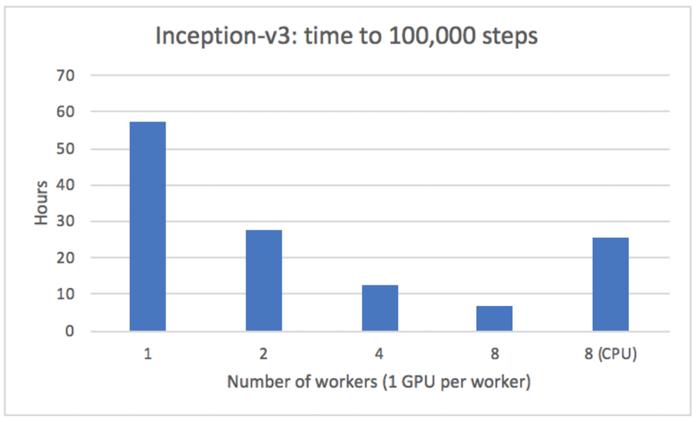
We ran the Inception v3 model on TonY with one to eight workers, with one GPU per worker (also one execution using CPU training on eight workers), using asynchronous training. This model is a well-known deep neural network for ImageNet, a dataset containing millions of images used for training image classification models. As in the Inception v3 distributed training example, we measured time to reach 100,000 steps with a batch size of 32. The results are below:
These results are with 40G RAM / 1 CPU per worker, Tesla K80 GPUs, on RHEL 6.6, and TensorFlow 1.9. The final top-5 error rate after reaching 100,000 steps for 8 workers with GPU training was 26.3%.
Since TonY is in the layer which orchestrates distributed TensorFlow and does not interfere with the actual execution of the TensorFlow job, we expect there to be no overhead. Indeed, we see that for GPU training, runtime scales linearly. We also see about four times speedup when running GPU training over CPU training, which is expected given the complexity and depth of the model.
In a tweet, Sam Altman said “It’s common to have a vision; it’s rare to plans.” This is so true. One problem though, what does it mean to have a plan?
Words that mean a lot of me from @sama, certainly the guiding words for me over many many projects. Problem-most people say they have plans (even after getting punched in the face) but they really don't have plans. So what is a plan, really? 1/
A plan is not “what are you going to do”. That’s still a vision. Most everyone thinks a plan is a detailed list of what you will get done reported in a kanban. One way to think about this is to first make sure you have a strategy, but what’s that?
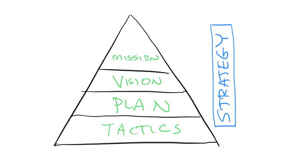
At the company level there is Mission, Vision, Plan, Tactics. See how plan is one part of this. Combine these and you have a strategy. Conflate them or fail to differentiate and you have a mess.
Hierarchy of Mission, Vision, Plan, Tactics that lead to a strategy. Source: author
Mission — how do we see the world as a better place b/c off what we do. Why do we exist. The world can be better for many reasons. World can mean “world of IT people struggling w/ X” as much as “cure a disease”, in this context. “Inspiration”. A mission is something that a company has.
Vision — Connect the mission to something concrete a product, service, goals that can be written down. Vision is aspiration. Visions can look like high fidelity visualizations (get it) articulated by design. A vision is something a product has.
Note: One trick is that the word “vision” is often used when speaker/listener are not in agreement on the time scale or level of abstraction. That’s the origin of this framework for me :-)
Plan — a plan is an operational framework that allows work to happen. It is an organization, resource allocation, set of processes. It is everything that determines success. More in a bit. A plan is a tool for creativity NOT a substitute for one.
Tactics — details of the plan at the individual or job function. The key thing about tactics is that the people doing the work own picking, executing, measuring them. Tactics include architecture, tools, dependencies, schedule, and more.
Only when you have all of these do you have a strategy. You might think you do but as the initial thread indicated, chances are you won’t execute. Now let’s double-click on a plan.
Key to plans, is (wait for it) PLANNING. Planning is a process. It takes time. It takes effort. It is not one assertive person dominating a channel or a whiteboard and gen’ing up a deck faster than anyone else. Plans are checks and balances against reality. For better or worse, plans are not “exciting”—the end result is exciting. True story: almost no exec I ever worked for was “excited” by a plan but could easily get excited by a demo.
A plan is like a news story. There is a lede, and then it goes on to say who, what, when, where, why, and how. But getting to this point requires iterating with the whole team/company so there is a shared understanding.
More than anything for a plan to be successful it needs to be shared.
STORY. Windows, Office used to have plans that would get distributed as memos to the whole team and also to the other teams (like Windows, Office, Tools, etc.) Planning itself is collaboration.
By the time we distributed those memos, themselves a product of several authors working together, the whole of the team was well-aware of not only the contents but their specific contribution (to the plan and then the product). Planning is working as a team.
Teams outside would see the memo and assume literally a single person (me?) just wrote the whole thing and it land on the team. The perception was that anything coherent and with so much detail had to be the work of one, not a “committee”. It was weird to me :-)
Part of the fun history here is that the team as a whole had absorbed the plan (and accountabilities associated with it) so others trying to tweek or randomize the plan would be met with a bit of “but we have a plan and understand what we’re doing”. Everyone wants to be an editor, it turns out (See Leading is Not Editing).
“Universally” there’s a perception/misunderstanding for plans to be both good and coherent they must come from one enlightened genius forcing it through a team. Likewise, any plan created by many people would be a sea of compromise.
That simply isn’t true. While in times of true crisis requiring instant action, one person can/must drive change, an execution plan taking years of the work of smart people needs to engage, enroll those smart people and early.
Genius plans are super rare. Teams are not.
Who. It might seem obvious, but first part of planning is making sure the right people are involved. At a startup you need to have sales involved early even if you think they will just accept the brilliance of the Eng team, for example.
What. What are the specific problems being solved? Not what are the features 1st. Starting from problems, then scenarios, and then a hierarchy of features. List your problems solved (X), scenarios (Y) and fill in a feature grid.
The what is an outline. It is almost always 3–5 “buckets” labeled with problems and then 3–5 “marquee” features. Marketing sees this and should think “I can turn this into positioning”. In fact the blog/PR writes itself.
When. Timing is life. Plans collapse when management (or sales) says now and prod/eng says 6 mon. and no one is entirely honest. Key: individuals doing work say how long. Key to a plan is leadership sets time constraint then work scales.
PS: If you’re coordinating plans across two orgs, then timing is the only universal language — and it is a language of commitment. Two teams can only work together if they share high integrity timing — two functional teams or client/back end, etc.
Where. Not geography it’s organizational statement. Who and what functions are responsible for what. Most startups don’t need to worry, but when big you align a team around a plan, not the other way. Remember, you will ship an org chart.
Why. Why for a plan is the definition of success. Will this create a new category, sustain the business, enable a new sales model, extend product in new directions, compete?
How. All along the team is deciding tools, architecture, processes to hit the ground running. Eng might test out a new runtime or tools. Finance/sales might iterate on pricing models <> features. Everyone is thinking execution cadence.
If you consider these and spend time to develop, you can write this down. In fact above is literally an outline of a memo. This memo is not “news” to the team, but distills the plan to a memo not just posterity but to insure “same page”.
Imagine having all this for when a new team member shows up. Not only do you tell them what to do, but they start being able to spend 20 minutes and know the whole backstory for what is going on. What a great recruiting tool too.
Developing robust algorithms for self-driving cars requires sourcing event data from over 10 billion hours of recorded driving time. But even with 10 billion-plus hours, it can be challenging to capture rare yet critical edge cases like weather events or collisions at scale. Luckily, these rare events can often be simulated effectively.
Cognata, a startup that develops an autonomous car simulator uses patented computer vision and deep learning algorithms to automatically generate a city-wide simulation that includes buildings, roads, lane marks, traffic signs, and even trees and bushes.
Simulating driving event data, however, requires expensive GPU and compute resources that vary depending on a given event. In working with Cognata, the big obstacle was going to be automation and creating on-demand resources in Azure.
In this code story, we’ll describe how we were able to provision custom GPU rendering clusters on demand with a Jenkins pipeline and Terraform.
The Challenges
Cognata required a scalable architecture to render its simulations across individual customers and events using GPU. To support this need, we first investigated using Docker containers and Kubernetes. However, at the time of this post, nvidia-docker does not officially support X server and OpenGL support is a beta feature. As an alternative to container orchestration, we architected a scalable solution using a GPU Azure Virtual Machine Scale Sets (VMSS) cluster and a custom application installation script for on-demand deployment.
The complex changesets must be applied to the infrastructure with minimal human interaction and must support building, changing, and versioning infrastructure safely and efficiently.
The solution
On-demand Infrastructure as Code
Cognata’s applications and services are deployed in a Kubernetes cluster and the rendering application is deployed in GPU Virtual machines clusters. To apply “Infrastructure as code” methodology, we decided to use Terraform and Jenkins.
Terraform allows us to provision, deprovision, and orchestrate immutable infrastructure in a declarative manner; meanwhile, Jenkins pipelines offers delivery process rather than an “opinionated” process and allows us to analyze and optimize the process.
Jenkins offered two big advantages:
The pipelines can be triggered via the HTTP API on demand.
Jenkins in Kubernetes is very easy. We used the Jenkins Helm chart:
$ helm install --name jenkins stable/jenkins
Deploying and Destroying resources
Creating on-demand resource required us to create detailed plans and specification of our resources. These plans are stored in a git repository such as GitHub or BitBucket to maintain versioning and continuity.
In our case, the plans included a Virtual Machines Scale Sets (VMSS) with GPU and an installation script of Cognata’s application. The VMSS was created from a predefined image that included all the drivers and prerequisites of the application.
Once we have the plans in the git repository, we need to run the workflow in the Jenkins pipeline to deploy the resources.
Starting the workflow can be triggered from an HTTP request to the Jenkins pipeline.
After the pipeline was triggered, the plans were pulled from the git repository and the deploying process is started using Terraform.
Terraform works in 3 stages:
Init – The terraform init command is used to initialize a working directory containing Terraform configuration files.
Plan – The terraform plan command is used to create an execution plan.
Apply – The terraform apply command is used to apply the changes required to reach the desired state of the configuration, or the pre-determined set of actions generated by a terraform plan execution plan.
Once the plan was executed and Terraform saved the state results in files, we needed to upload the result files to a persistent storage such as Azure Blob storage . This step would later enable us to download the state files and destroy the resources that we created after the business process was completed, and to actually create on-demand clusters.
The flow of the solution is described in the following image:
Terraform client
To invoke Terraform commands in the Jenkins pipeline, we created a small Docker container with Terraform and Azure CLI with the following Dockerfile.
With the adoption of driverless cars, 10 billion-plus hours of recorded driving time just isn’t viable. Cognata’s complex simulations rendering for multiple autonomous car manufacturers can become costly and inefficient. Our Jenkins pipeline and Terraform solution enabled Cognata to dynamically scale GPU resources for their simulations, making it easier to serve their customers while saving significant cost in compute resources. Using these technologies we were able to automate the deployment and maintenance of Cognata’s Azure VMSS GPU clusters and simulation logic.
Our joint solution is adaptable to any workload that requires:
Provisioning Azure resources using Terraform.
Using the Jenkins DevOps process to provision on-demand resources in Azure and in Kubernetes.
We recently worked with a financial services partner to develop a model to predict the future stock market performance of public companies in categories where they invest. The goal was to use select text narrative sections from publicly available earnings release documents to predict and alert their analysts to investment opportunities and risks. We developed a deep learning model using a one-dimensional convolutional neural network (a 1D CNN) based on text extracted from public financial statements from these companies to make these predictions. We used Azure Machine Learning Workbench to explore the data and develop the model. We modeled our solution using the Keras deep learning Python framework with a Theano backend. Our results demonstrate how a deep learning model trained on text in earnings releases and other sources could provide a valuable signal to an investment decision maker.
The Challenge
When reviewing investment decisions, a firm needs to utilize all possible information, starting with publicly available documents like 10-K reports. However, reviewing public earnings release documents is time-intensive and the resulting analysis can be subjective. Moreover, the written sections of an earnings release require the most review time and are often the most subjective to interpretation. A thorough analysis of the investment opportunity of a business would also include a review of other companies in the industry to understand relative performance. Our challenge was to build a predictive model that could do a preliminary review of these documents more consistently and economically, allowing investment analysts to focus their follow-up analysis time more efficiently and resulting in better investment decisions.
For this project, we sought to prototype a predictive model to render consistent judgments on a company’s future prospects, based on the written textual sections of public earnings releases extracted from 10k releases and actual stock market performance. We leveraged natural language processing (NLP) pre-processing and deep learning against this source text. In the end, we sought a model that was easy to operationalize, use and maintain over time. While there are broader potential applications of processing public earnings release narratives to predict future stock value, for the purposes of this project we focused just on generating predictions that could better inform further human analysis by our partner.
Our Approach
Tooling, Pre-Processing and Initial NLP Exploration
We began our work in Python with Azure Machine Learning Workbench, exploring our data with the aid of the integrated Jupyter Notebook. We used the base AML Workbench Python libraries, including NLTK, and added some additional packages and NLP tools including the Gensim library. All scripts and sample data are available in this GitHub repo, including Jupyter Notebooks for each of the steps, from filtering source data to pre-processing, running and evaluating the model. To make things easier, you’ll find a list of the Python packages and utilities to install on top of the base Azure Machine Learning Workbench Python installation listed in the readme.
As input, we gathered a text corpus of two years of earnings release information for thousands of public companies worldwide. We extracted as source the sections 1, 1A, 7 and 7A from each company’s 10k — the business discussion, management overview, and disclosure of risks and market risks. We also gathered the stock price of each of the companies on the day of the earnings release and the stock price four weeks later. We categorized the public companies by industry category.
We pre-processed the text, converting to UTF-8, removing punctuation, stop words, and any character strings less than 2 characters. The pre-processing Jupyter Notebooks are on GitHub (Source Text Filtering and Text Cleaning). Many of the techniques we used are described in detail in the NLTK in Python book. Below is an example of cleaned text, which in this case is a sample of a management overview from one earnings release. A number of text document samples are available on GitHub.
business overview acad overview we are biopharmaceutical company focused discovery development commercialization small molecule drugs treatment central nervous system disorders we currently have six clinical programs several additional programs discovery development our most advanced program we are conducting phase iii studies pimavanserin treatment parkinson disease psychosis we have reported positive results phase ii trial our program pimavanserin co therapy schizophrenia we also have completed enrollment phase iib trial our program acp stand alone treatment schizophrenia addition we have completed proof concept clinical study pimavanserin treatment sleep maintenance insomnia healthy older adults we have retained worldwide
An important consideration in our approach was our limited data sample of less than 35,000 individual text document samples across industries, with much smaller sample sizes within an industry. Within biotechnology, we had 943 text document samples. As a result of the sample limitations, our project results should be viewed as simply a proof of concept to be validated and improved with additional samples.
Another factor was the large amounts of industry-specific vocabularies contained in each of the text documents. To better understand the variation within the corpus, we cleaned the text the help of NLP methods and libraries including NLTK and Gensim. When inspecting the source text from public company releases with an LDA topic model analysis, we found that there was a large amount of vocabulary variation between industry vocabularies, and much less variability within industries. This finding led us to prototype our performance classification model based on single industries, rather than across them, in order to reduce the amount of less meaningful variation noise. The Jupyter Notebook details the initial text exploration in the Jupyter Notebooks folder.
Representing Documents as Word Vectors
In order to take advantage of NLP deep learning, we needed to obtain numerical representation for our text. Specifically, we needed vector representations for each of our documents. Natural language, by its nature, has localized spatial correlations between words. For example, if you find the word ‘sunny’, you may be more likely to find the word ‘weather’ in the same sentence than another less closely related word. Word vector models represent these relationships numerically. In particular, word embedding is a technique wherein word pairs can be represented based on the Euclidian distance between them which can encode the semantic differences and similarities. These distances can be represented by vector differences.
There were two options for creating word embeddings. We could create custom embeddings based on our corpus of source texts, or we could leverage a pre-trained model based on a much larger corpus of text. Given the limited size of our sample, we looked to leveraged pre-trained word vectors. In our case, we used GloVe pre-trained models. These pre-trained models were trained on aggregate global word-word co-occurrence from a variety of very large datasets. The result is a vector that represents the linear substructure of the word vector space. We used the GloVe pre-trained model of all of Wikipedia’s 2014 data, a six billion token, 400,000-word vocabulary vector model, chosen for its broad domain coverage and less colloquial nature. This pre-trained set of word vectors allowed us to vectorize our document set and prepare it for deep learning toolkits.
Word Vector Example
Although this pre-trained model has a vast 400,000-word vocabulary, it still has limitations as it relates to our text corpus. For example, in technology-driven industries, there is a highly specialized, domain-specific vocabulary which may not be represented in the pre-trained word model. These vocabulary terms might be predictive of performance, but when we used these pre-trained word models, out-of-vocabulary words would all get the same word vector values which reduce their predictive value. For some industries, this vocabulary changes over time as new technologies, compounds or products are developed. As a result, the word vector of these changing words might need to be different at different periods of time. The presence of the newest technology vocabulary might also have predictive value. In addition, the corporate earnings release statements are rendered with a particular subtle patois not fully reflected in the Glove model pre-trained on Wikipedia articles.
Research is emerging on new methods for dealing with out of vocabulary words for small vocabularies, and the temporal dimension of vocabulary words. This post sums up important recent NLP research which promises to solve these issues in the future.
Classification Labels and Prediction Goal
We created three equally sized classification bins of high, medium and low performance based on the performance of the stock between the date of the release and four weeks later. The performance was calculated as the percentage change in the stock value in that time and applied some normalization for overall stock market changes. These low, medium and high 4-week performance classifications were the labels in our model. We modeled our prototype on just one industry, the biotechnology industry, which had the most abundant within-industry sample. Our project goal was to discern whether we could outperform chance accuracy of 33.33%.
Convolutional Neural Net Model with Keras
With our documents represented by a series of embeddings, we were able to take advantage of a convolutional neural network (CNN) model to learn the classifications. CNNs can be well suited to document modeling, as they can find small (and then large) syntactic structures across the training set through convolutional and max pooling steps, building a fuller model of the source corpus (read more about CNNs with NLP). Below is a depiction of a one layer CNN. With our limited sample of source documents and very limited timespan of our data points, we chose the simpler 1D CNN, rather than using an LSTM model for this project.
We used a 1D CNN in Keras using our custom word embeddings. See this excellent Keras example for a 1D CNN architecture using custom word embeddings, like those pre-trained Glove model word vectors. In our model design, we started from the Keras reference as our architectural base and refined from there.
We chose a 10,000-word sequence as the maximum. For those documents with more than 10,000 words, we truncated the remaining text. For those documents with fewer than 10,000 words, we padded the sequence at the end with zeroes. We mapped each of our words in each sequence to one of the Glove embedding vocabulary items and used its 300 value numerical representation. For each document sample, we had a 10,000 x 300 sequence representation. Below is an excerpt of building the embedding matrix from this script.
#################################
#Build the embedding matrix
#################################

print('Building Embedding Matrix...')
embedding_matrix = np.zeros((len(word_index) + 1, EMBEDDING_DIM))
for word, i in word_index.items():
    embedding_vector = embeddings_index.get(word)
    if embedding_vector is not None:
        # words not found in embedding index will be all-zeros.
        embedding_matrix[i] = embedding_vector

embedding_layer = Embedding(len(word_index) + 1,
                            EMBEDDING_DIM,
                            weights=[embedding_matrix],
                            input_length=MAX_SEQUENCE_LENGTH,
                            trainable=False)
For the model itself, we employed the ADAM optimizer, the Lecuninitializer, and we used exponential linear unit (‘elu’)activation function. We applied dropout in training (15% to inner layers, and 45% to the final layer), and the Keras early stopping feature to prevent over-fitting. Also, we stepped down the learning rate from the initial model to improve the test results to .00011. We discovered the model was very sensitive to initializer choices, with the Lecun model offering much better learning than other all other initializers available in Keras. After testing all the optimizer options in Keras, we found that both ADAM and RMSprop optimizers performed much better than other optimizers, with ADAM performing slightly better. When we used the ‘elu’ function, the model trained less erratically than with the Relu, Prelu or Leaky Relu activation functions, and reached higher accuracy. We stepped down batch size to a modest size of 33 to improve learning.
In order to improve the model, we augmented the data in the original text with the title of the section from the 10-K report. We appended this text to the start of the document sample. Thesaurus-based data augmentation in NLP is discussed in more depth in this forum discussion.
########################
#Select Model Parameters
########################
MAX_SEQUENCE_LENGTH = 10000 #Max sequence of 10k words from each sample
MAX_NB_WORDS = 400000 #Using the full Glove Vocabulary
EMBEDDING_DIM = 300 #Each word in the sequence represented by 300 values
VALIDATION_SPLIT = 0.2  #Train/Test Split
LEARNING_RATE = .00011
BATCH_SIZE = 33
DROPOUT_RATE = 0.45  #Dropout applied to last layer
INNERLAYER_DROPOUT_RATE = 0.15  #Dropout applied to inner layers

##############
#1D CNN DESIGN
##############
sequence_input = Input(shape=(MAX_SEQUENCE_LENGTH,), dtype='int32')

embedded_sequences = embedding_layer(sequence_input)

x = Conv1D(128, 5, activation='elu', kernel_initializer='lecun_uniform')(embedded_sequences)
x = MaxPooling1D(5)(x)
x = Dropout(INNERLAYER_DROPOUT_RATE)(x)

x = Conv1D(128, 5, activation='elu', kernel_initializer='lecun_uniform')(x)
x = MaxPooling1D(5)(x)
x = Dropout(INNERLAYER_DROPOUT_RATE)(x)

x = Conv1D(128, 5, activation='elu', kernel_initializer='lecun_uniform')(x)
x = MaxPooling1D(35)(x)  # global max pooling

x = Flatten()(x)
x = Dense(100, activation='elu', kernel_initializer='lecun_uniform')(x) # best initializers: #glorot_normal #VarianceScaling #lecun_uniform
x = Dropout(DROPOUT_RATE)(x)

preds = Dense(len(labels_index), activation='softmax')(x) #no initialization in output layer

model = Model(sequence_input, preds)
The Result
Our prototype model results, while modest, suggest there is a useful signal available on future performance classification in at least the biotechnology industry based on the target text from the 10-K. The resulting statistics are listed below, including the statistics by class. For our model, ‘0’ represents low performance, ‘1’ represents middle performance and ‘2’ represents high performance (see model evaluation notebook).
The confusion matrix below details the prediction comparing the true class of the sample, and the predicted class. The true label is on the vertical axis, and the predicted label coming from our model is on the horizontal axis. The top grid is the absolute count, and the bottom grid is the percentage. The visualization shows that our model performs best at predicting the true label of the low performing stocks, in the upper left.
For investment firms, predicting likely under-performers may be the most valuable prediction of all, allowing them to avoid losses on investments that will not fare well. Chance would have given us a 33.3% accuracy for any one classification. In this model, we are seeing 62% accuracy for predicting the under-performing company based on the sample 10-K text.
The history of model training and testing is below, trained for 24 epochs.
Next Steps
This initial result suggests that that deep learning models trained on text in earnings releases and other sources could prove a viable mechanism to improve the quality of the information available to those making investment decisions, particularly in avoiding investment losses. While the model needs to be improved with more samples, refinements of domain-specific vocabulary, and text augmentation, it suggests that providing this signal as another decision input for investment analyst would improve the efficiency of the firm’s analysis work.
Our partner will look to improve the model with more samples and to augment them with additional information taken from the earnings releases and additional publications and a larger sample of companies. They will also explore alternative model architectures including LSTM to better understand the sequential nature of the publication and performance information. In addition, they will look to replicate this model for different industries and operationalize the model with Azure Machine Learning Workbench, allowing auto-scaling and custom model management for many clients.
Overall, this prototype validated additional investment by our partner in natural language based deep learning to improve efficiency, consistency, and effectiveness of human reviews of textual reports and information. Please feel free to reach out in comments below or directly via Twitter @SingingData.
This is the first part of a 2 part blog series. In this series we will talk about Scio, a Scala API for Apache Beam and Google Cloud Dataflow, and how we built the majority of our new data pipelines on Google Cloud with Scio.
Scio > Ecclesiastical Latin IPA: /ˈʃi.o/, [ˈʃiː.o], [ˈʃi.i̯o] > Verb: I can, know, understand, have knowledge.
Introduction
Over the past couple of years, Spotify has been migrating our infrastructure from on premise to Google Cloud. One key consideration was Google’s unique offerings of high quality big data products, including Dataflow, BigQuery, Bigtable, Pub/Sub and many more.
Google released Cloud Dataflow in early 2015 (VLDB paper), as a cloud product based on FlumeJava and MillWheel,two Google internal systems for batch and streaming data processing. Dataflow introduced a unified model to batch and streaming that consolidates ideas from these previous systems, and the Google later donated the model and SDK code to the Apache Software Foundation as Apache Beam. With Beam, an end user can build a pipeline using one of the SDKs (currently Java and Python), which gets executed by a runner for one of the supported distributed systems, including Apache Apex, Apache Flink, Apache Spark and Google Cloud Dataflow.
Scio is a high level Scala API for the Beam Java SDK created by Spotify to run both batch and streaming pipelines at scale. We run Scio mainly on the Google Cloud Dataflow runner, a fully managed service, and process data stored in various systems including most Google Cloud products, HDFS, Cassandra, Elasticsearch, PostgreSQL and more. We announced Scio at GCPNEXT16 last March and it’s been gaining traction ever since. It is now the preferred data processing framework within Spotify and has gained many external users and open source contributors.
In this first post we will take a look at the history of big data at Spotify, the Beam unified batch and streaming model, and how Scio + Beam + Dataflow compares to the other tools we’ve been using. In the second post we will look at the basics of Scio, its unique features, and some concrete use cases at Spotify.
Big Data at Spotify
At Spotify we process a lot of data for various reasons, including business reporting, music recommendation, ad serving and artist insights. We serve billions of streams in 61 different markets and add thousands of new tracks to our catalogue every day. To handle this massive inflow of data, we have a ~2500 node on-premise Apache Hadoop cluster, one of the largest deployments in Europe, that runs more than 20K jobs a day.
Spotify started as a Python shop. We created Luigi for both job orchestration and Python MapReduce jobs via Hadoop streaming. As we matured in data processing, we began to use a lot of Scalding for batch processing. Scalding is a Scala API from Twitter that runs on Cascading, a high-level Java library for Hadoop MapReduce. It allows us to write concise pipelines with significant performance improvement over Python. The type-safe functional paradigm also boosts our confidence in code quality and correctness. Discover Weekly, one of our very popular features, is powered by Scalding (BDS2015 talk). We also use Apache Spark for some machine learning applications, leveraging its in-memory caching capability for iterative algorithms.
On the streaming side we’ve been using Apache Storm for a few years now to power real time use cases like new user recommendation, ads targeting and product metrics. Most pipelines are fairly simple, consuming events from Apache Kafka, performing simple filtering, aggregation, metadata lookups, and saving output to Apache Cassandra or Elasticsearch. The Storm API is fairly low level which limited its application for complex pipelines. We’ve since moved from Kafka to Google Cloud PubSub for ease of operations and scaling.
Apart from batch and streaming data processing, we also do a lot of ad-hoc analysis using Hive. Hive allows business analysts and product managers to analyze huge amounts of data easily with SQL-like queries. However Hive queries are translated into MapReduce jobs which incur a lot of IO overhead. On top of that we store most of our data in row-oriented Avro files which means any query, regardless of actual columns selected, requires a full scan of all input files. We migrated some core datasets to Apache Parquet, a columnar storage format based on Google’s Dremel paper. We’ve seen many processing jobs gaining 5-10x speed up when reading from Parquet. However support in both Hive and Scalding has some rough edges and limited its adoption. We’ve since moved to Google BigQuery for most ad-hoc query use cases and have experienced dramatic improvements in productivity. BigQuery integration in Scio is also one of its most popular features which we’ll cover in the second part.
Beam Model
Apache Beam is a new top level Apache project for unified batch and streaming data processing. It was known as Google Cloud Dataflow before Google donated the model and SDK code to the Apache Software Foundation. Before Beam the world of large scale data processing was divided into two approaches: batch and streaming. Batch systems, e.g. Hadoop map/reduce, Hive, treat data as immutable, discrete chunks, e.g. hourly or daily buckets, and process them as a single unit. Streaming systems, e.g. Storm, Samza, process continuous streams of events as soon as possible. There is prior work on unifying the two, like the Lambda and Kappa architectures, but none which address the different mechanics and semantics in batch and streaming systems.
Beam implements a new unified programming model for batch and streaming introduced in the Dataflow paper. In this model, batch is treated as a special case of streaming. Each element in the system has an implicit timestamp and window assignment. In streaming mode, the system consumes from unbounded (infinite and continuous) sources. Events are assigned timestamps at creation (event time) and windowed, e.g. fixed or sliding window. In traditional batch mode, elements are consumed from bounded (finite and discrete) sources and assigned to the same global window. Timestamps usually reflect the data being processed, i.e. hourly or daily bucket.
Beam Model
This model also abstracts parallel data processing as two primitive operations, parallel do (ParDo) and group by key (GBK). ParDo, as the name suggests, processes elements independently in parallel. It is the primitive behind map, flatMap, filter, etc. and behaves the same in either batch or streaming mode. GBK shuffles key-value pairs on a per window basis to collocate the same keys on the same workers and powers groupBy, join, cogroup, etc. In the streaming model, grouping happens as soon as elements in a window are ready for processing. In batch mode with single global window, all pairs are shuffled in the same step.
With this simple yet powerful abstraction, one can write truly unified batch and streaming pipelines in the same API. We can develop against sampled log files, parsing timestamps and assigning windows to log lines in batch mode, and later run the same pipeline in streaming mode using Pub/Sub input with little code change. Checkout Beam’s mobile gaming examples for a complete set of batch + streaming pipeline use cases.
Enter Scio
We built Scio as a Scala API for Apache Beam’s Java SDK and took heavy inspiration from Scalding and Spark. Scala is the preferred programming language for data processing at Spotify for three reasons:
Good balance between productivity and performance. Pipeline code written in Scala are usually 20% the size of their Java counterparts while offering comparable performance and big improvement over Python.
Access to large ecosystem of both infrastructure libraries in Java e.g. Hadoop, Beam, Avro, Parquet and high level numerical processing libraries in Scala like Algebird and Breeze.
Functional and type-safe code is easy to reason about, test and refactor. These are important factors in pipeline correctness and developer confidence.
In our experience, Scalding or Spark developers can usually pick up Scio without any training while those from Python or R background usually become productive within a few weeks and many enjoy the confidence boost from functional and type-safe programming.
So apart from the similar API, how does Scio compare to Scalding and Spark? Here are some observations from different perspectives.
Programming model
Spark supports both batch and streaming, but in separate APIs. Spark supports in-memory caching and dynamic execution driven by the master node. These features make it great for iterative machine learning algorithms. On the other hand it’s also hard to tune at our scale.
Scalding supports batch only and there’s no in-memory caching or iterative algorithm support. Summingbird is another Twitter project that supports batch + streaming using Scalding + Storm. But this also means operating two complex systems.
Scio supports both batch and streaming in the same API. There’s no in-memory caching or iterative algorithm support like Spark but since we don’t use Scio mainly for ML it has not been a problem.
Operational modes
With Spark, Scalding, Storm, etc. you generally need to operate the infrastructure and manage resources yourself, and at Spotify’s scale this usually means a full team. Deploying and running code often requires both knowledge of the programming model and the infrastructure you’re running it on. While there are services like Google Cloud DataProc and similar Hadoop-as-a-Service products, they still require some administrative know-how to run in a scalable and cost-effective manner. Spydra and Netflix’s Genie are some examples of additional tooling for such operation.
Scio on Google Cloud Dataflow is fully managed, which means there is no operational overhead of setting up, tear down or maintaining a cluster. Dataflow supports auto-scaling and dynamic work rebalancing which makes the jobs more elastic in terms of resource utilization. A data engineer can write code and deploy from laptop to the cloud at scale without any operational experience.
Google Cloud Integration
While there are Hadoop connectors for GCS, BigQuery, plus native clients for several other products, the integration of these with Scalding and Spark is nowhere near as seamless as that of Dataflow.
This is where Dataflow shines. Being a Google project, it comes with connectors for most Google Cloud big data projects, including Cloud Storage, Pub/Sub, BigQuery, Bigtable, Datastore, and Spanner. One can easily build pipelines that leverage these products.
By moving to Scio, we are simplifying our inventory of libraries and systems to maintain. Instead of managing Hadoop, Scalding, Spark and Storm, we can now run the majority of our workloads with a single system, with little operational overhead. Replacing other components of our big data ecosystem with managed services, e.g. Kafka with Pub/Sub, Hive with BigQuery, Cassandra with Bigtable, further reduces our development and support cost.
This concludes the first part of this blog series. In the next part we’ll take a closer look at Scio and its use cases. Stay tuned.
Lots of people have raised small VC funds. There are more startups, and there’s more LP capital from various sources to meet that demand. After the rise of institutional seed funds in the late 2000’s, we’ve obviously witnessed a pure explosion of new (mostly seed) fund formation, with seemingly no end in sight. Many of those 400+ microVC funds (sub $100M) are also trying not only get bigger, but also trying to convert their LP capital base from mostly individuals to mostly traditionally institutional capital. It’s a heavy lift to make that conversion. While I would never give advice on how to do this, as I’m still learning and each individual case is very different (each fund manager is his/her own special snowflake!), I can share a bit about how I prepared myself for it, how I launched my campaign, and how it all closed. My hope is that this post serves as a helpful guidepost for other managers and that it can save someone time in the future. Much of this below benefits from me looking back with hindsight… there’s lots in here that I wish I had known just a year ago!
At a high level, I break this process into three distinct phases: (1) Pre-Marketing Preparations; (2) The Actual Campaign; and (3) The Closing Mechanics.
Phase 1: Pre-Marketing Preparations
Timing: I built my LP list and began putting the word out two months before hitting the market. Now looking back, i wish I pre-marketed a full six months in advance. Institutional LPs need lots of time to meet folks, to digest initial meetings, to socialize things with their network, and to fill their pipeline. I could even argue that six months is too short. During these meetings, it’s nice to socialize your plans, target size, and strategy. LPs will offer great feedback which can be refined and folded into your final official campaign.
Materials: i prepared a master slide deck (with the help of a designer that I paid REAL money to), which I sliced into a very short “email deck” and a slightly longer “presentation deck.” In retrospect, I only needed the shorter deck (to get the meeting, and for LPs to circulate to their colleagues and peers). I sent everything via PDF, with no exception. What mattered most in the materials was explaining the manager’s background & differentiation (what makes you stand out?, the strategy (where to invest the fund), the portfolio construction (how to invest the fund), deal sourcing (where do you get your leads from). I’ll go into more details on this in future posts.
Key Service Providers: I signed up with very well-known and vetted legal counsel in fund formation, fund administration (back office), and banking. For me, finally being able to go with the top class players forced me to play a better game.
LPA Documents: I asked legal counsel to make my fund docs “plain vanilla,” very simple and in-line with the market. I am not a proven manager. I was shocked to hear how many people play games with the LPA when they haven’t returned real capital.
Data Room: I built a data room on Box with a paid subscription. The folders in my Box data room covered the following topics: References (co-investors, follow-on VCs, previous LPs, and portfolio CEOs); Press Mentions; Notable Blog Posts; Raw Investment Data; Service Providers; Marketing Materials; Previous LP Reports; Audit Paperwork; Official Fund Documentation. The file formats in my Box data room were only PDF, .xls, .jpg, and .png.
Lead Qualification & Tools: The pre-marketing campaign is a good time to find out who isn’t a fit. I had a friend who is an LP just tell me even before seeing the deck or anything that it wouldn’t be a fit. He actually helped me a ton in my process. Similarly, I was able to get into the pipeline of other LPs as I hit the market. I managed my contacts and flow through Pipedrive.
Skin In The Game: LPs will look for any new manager to commit a raw dollar amount commensurate with their liquid net worth. To be safe, I would suspect 2% GP commit would be table stakes, and many folks have to finance that. For folks who have the nest egg, wise to expect to put the appropriate skin in the game.
Phase 2: The Actual Campaign
I will just briefly share what I did. I think it is different for everyone. If anything, I would be conservative in how long you think it will take — and then add another 3-6 months to that conservative projection.
At a high-level, I made three initial decisions that, again in retrospect, made (I believe) a big difference — however, it didn’t feel that way until the very end. Specifically, I picked a tight target size range and I stuck with it — I never once entertained going one dollar over the high-end of my target. Two, I told everyone that I’d be “in market” for six months, and that’s it. No special closes. No opening the fund for even the most royal LPs after it was closed. Third, I told everyone that whatever I had at the end of six months would be my fund size and I would fight the war with the army I had, even if it was well below my target. I don’t know why I stuck to this all the way through, but it is what I believed in and I basically ran out of gas as the sixth month came to an end, so it was good to know I was going to stop then.
I put my rear on an airplane. A lot. I flew over 40,000 miles (all in the U.S.). I spent 28 nights away from home, two of them as red-eyes. I probably talked with and had initial calls/meetings with over 200 different institutional LPs. Naturally, most didn’t go to a second live meeting, but more than enough did. I did not wait until an LP was going to be in the Bay Area to see them — they’re usually only here for a night or two, at the most, and they have to see their current managers. I went to see them on their turf, every single time. I took notes in every meeting. I have a pretty good sense now of what LPs are in specific VC funds. Note-taking is important to remember follow-ups, to understand their network and relationship, and to send them things that interest them in their business. As they get more interested in you, they will come meet you in neutral locations or on your turf, and those signals are important markers to pay attention to.
The entire decision often rests on the quality of your references. It is very hard to quickly gin up references. You either have stellar references or you don’t. Even your biggest supporters will share your weaknesses and area for improvement with prospective LPs. Even though I’ve now raised four different funds, I couldn’t believe how much referencing went on this time. There is nowhere to hide. However you’ve treated others and behaved, it will be surfaced — for better or worse. LPs are looking at the history
It sounds corny, but I befriended a good deal of LPs who passed on me very quickly but were so nice and helpful (as people) that i sent them tips on new interesting funds and managers, some of which even led to them making an LP investment. Once you accept that most LPs are decent people and that they’re going to say “no,” it becomes easier to simply have a conversation with them. Some of them are really far away from our world of startups and VC funds; yet, some of them are incredibly deep into it and know way much more than even popular fund managers do. Sure, there will be some that you meet that you hope to never see again, but it’s a very small minority.
I held two official closes. The first close was half-way through the campaign, and most of my insiders re-upped and some super-sized. Looking back, I thought I would have more of the fund done by then — but, no, not even close. In the second-half of the campaign, I turned on the jets and just focused on the institutions. Seven business days before I was set to give it up and go with what I had, I finally got a string of institutional LP commits, like dominoes falling. It was really random. If you follow NBA history, it was like the Pacers-Knicks game where Reggie Miller hit all those three-pointers at the end. It felt like that. I got lucky, but it was really close.
Phase 3: The Closing Mechanics
I only can share some high-level learnings here:
1/ Good legal counsel matters. It is an art to line up these different LPs at the same time and on the same terms.
2/ No one but you has the deep urgency to close. You have to be fierce in pursuit of the close. Some people will get annoyed with it, but you have to close it out.
3/ Expect a major curveball. I can’t say what it will be, but expect to be taken by surprise and roll with it.
[Big disclaimer — I cannot emphasize enough how many people you will need to help you and advocate for you to get over the finish line. I have been in awe of what others have done for me. All the reference calls, extra nudges over text, and pounding the table even in cases when it didn’t work out. I will go through this process and thank folks properly in the coming weeks.]
I hope this helps folks out there. I hope you’ll notice this isn’t as detailed as it could be. I think the process can be pretty simple and straightforward. Set up the materials properly, be human in the meetings, follow-up with precision, and drive people to a decision and close. Lots of folks have been asking me recently “How did you do it?” so I thought it would be only fair for me to share it more broadly and expand on key areas over the next few weeks. Good luck out there!